Statistics provides tools and methods to find structure and to give deeper data insights. Both Statistics and Mathematics love facts and hate guesses. Knowing the fundamentals of these two important subjects will allow you to think critically, and be creative when using the data to solve business problems and make data-driven decisions.

So in simple terms:

“Statistics is the grammar of science.” Karl Pearson

Let's get into this,

Sample and Population

Suppose you have a dataset of a company having 56k employees, when you are taking out 10k random rows from that data that is a sample when you are considering all 56k rows its population

Statistics have majorly been categorized into two types:

1. Descriptive statistics (summarizes or describes the characteristics of a data set.)

2. Inferential statistics (you take out sample from data(also called population) to describe and make inferences about the population.)

Descriptive statistics consists of two basic categories of measures:

1. measures of central tendency (Mean, Median, Mode)

2. measures of variability or spread (Standard Deviation, variance, range)

Where Measures of central tendency describe the center of a data set.

Measures of variability or spread describe the dispersion of data within the set.

Inferential statistics

Inferential statistics is all about taking a sample and conducting appropriate tests. key tests in Inferential statistics are Hypothesis testing Z-test T-test Chi-square test Anova

Difference between Descriptive statistics and Inferential statistics

In Descriptive statistics, you take the data or population and further analyze, Visualize and summarize the data in form of numbers and graphs.

On the other side in Inferential statistics, we take the sample of the population do some tests to come up with inferences and conclusions about that particular population.

Random Variables

A random variable is a numerical description of the outcome of a statistical experiment.

Consider the experiment of tossing two coins. We can define X to be a random variable that measures the number of heads observed in the experiment. For the experiment, the sample space is shown below:

S = {(H, H), (H, T), (T, H),(T, T)}

There are 4 possible outcomes for the experiment, and this is the domain of X. The random variable X takes these 4 outcomes/events and processes them to give different real values. For each outcome, the associated value is shown as:

X(H, H) = 2 (two heads)
X(H, T) = 1 (one head)
X(T, H) = 1 (one head)
X(T, T) = 0 (no heads)

There are three types of random variables- discrete random variables, continuous random variables, and mixed random variables.

Discrete- Discrete random variables are random variables, whose range is a countable set. A countable set can be either a finite set or a countably infinite set. Eg: Bank Account number in a random group.

Continuous- Continuous random variables, on the contrary, have a range in the forms of some interval, bounded or unbounded, of the real line. E.g., Let Y be a random variable that is equal to the height of different people in a given population set.

Mixed Random Variables: Lastly, mixed random variables are ones that are a mixture of both continuous and discrete variables.

Mean, Median, Mode Explained

Mean: is the sum of all observations divided by the number of observations. Mean is denoted by x̄ (pronounced as x bar). also μ pronounced “mew”

Median: The value of the middlemost observation, obtained after arranging the data in ascending order, is called the median of the data.

Why/Where median is used: if there are outliers in your data mean represents a different form of distribution and it is harmful to analysis.

height=[10,20,30,40,50,10000]
print(np.mean(height))
print(np.median(height))

#output: 
#1691.6666666666667
#35.0

For instance, in the above example, there is a significant difference in mean and median with only a single outlier. so median is used in such cases to find central tendency.

Mode: The value which appears most often in the given data i.e. the observation with the highest frequency is called a mode of data.

# calculating mean median and mode in python
import numpy as np
from scipy import stats

# sample of height in cms
sample_of_height= [145,170,160,182,142,175,149,143,161,148,155,158,145,145]
print(np.mean(sample_of_height))
print(np.median(sample_of_height))
print(stats.mode(sample_of_height))

Measure of dispersion:

Range: Range, stated simply, is the difference between the largest (L) and smallest (S) value of the data in a data set. It is the simplest measure of dispersion.

Quartiles: are special percentiles, which divide the data into quarters.

The first quartile, Q1, is the same as the 25th percentile,

The median is called both the second quartile, Q2, and the 50th percentile.

and the third quartile, Q3, is the same as the 75th percentile.

Interquartile Range (IQR) The IQR is a number that indicates how spread the middle half (i.e. the middle 50%) of the dataset is and can help determine outliers. It is the difference between Q3 and Q1.

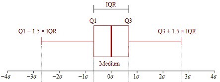
Understanding Interquartile Range (IQR) with boxplot

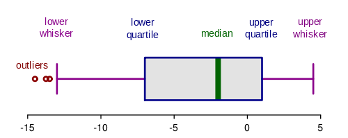
Generally speaking, outliers are those data points that fall outside of the lower whisker and upper whisker.

Standard Deviation: measures the dispersion of a dataset relative to its mean. denoted by symbol σ Standard Deviation is the square root of the variance.

Variance: Variance is a measurement of the spread between numbers in a data set. denoted by symbol σ2 (Square of Standard Deviation)

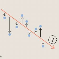
variance is used to see how individual numbers relate to each other within a data set.

Normal Distribution (also called Gaussian distribution)

Values that are symmetric about the mean, showing that data near the mean are more frequent in occurrence than data far from the mean. Normal distributions are symmetrical, but not all symmetrical distributions are normal.

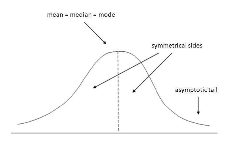
Empirical rule in normal distribution:

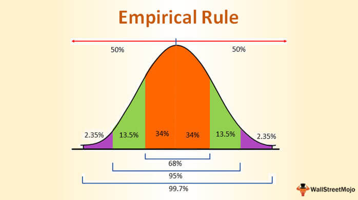
The empirical rule also referred to as the three-sigma rule or 68-95-99.7 rule, is a statistical rule which states that for a normal distribution, almost all observed data will fall within three standard deviations

In particular, the empirical rule predicts that

68% of observations fall within the first standard deviation (µ ± σ),

95% within the first two standard deviations (µ ± 2σ), and

99.7% within the first three standard deviations (µ ± 3σ).

Central Limit Theorem:

The central limit theorem states that the sampling distribution of the mean approaches a normal distribution, as the sample size increases. This fact holds especially true for sample sizes over 30.

for better understanding watch this.

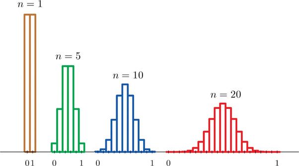
Here n= number of observations, as n increases distribution starts looking like a normal distribution.

The central limit theorem tells us that no matter what the distribution of the population is, the shape of the sampling distribution will approach normality as the sample size (N) increases.

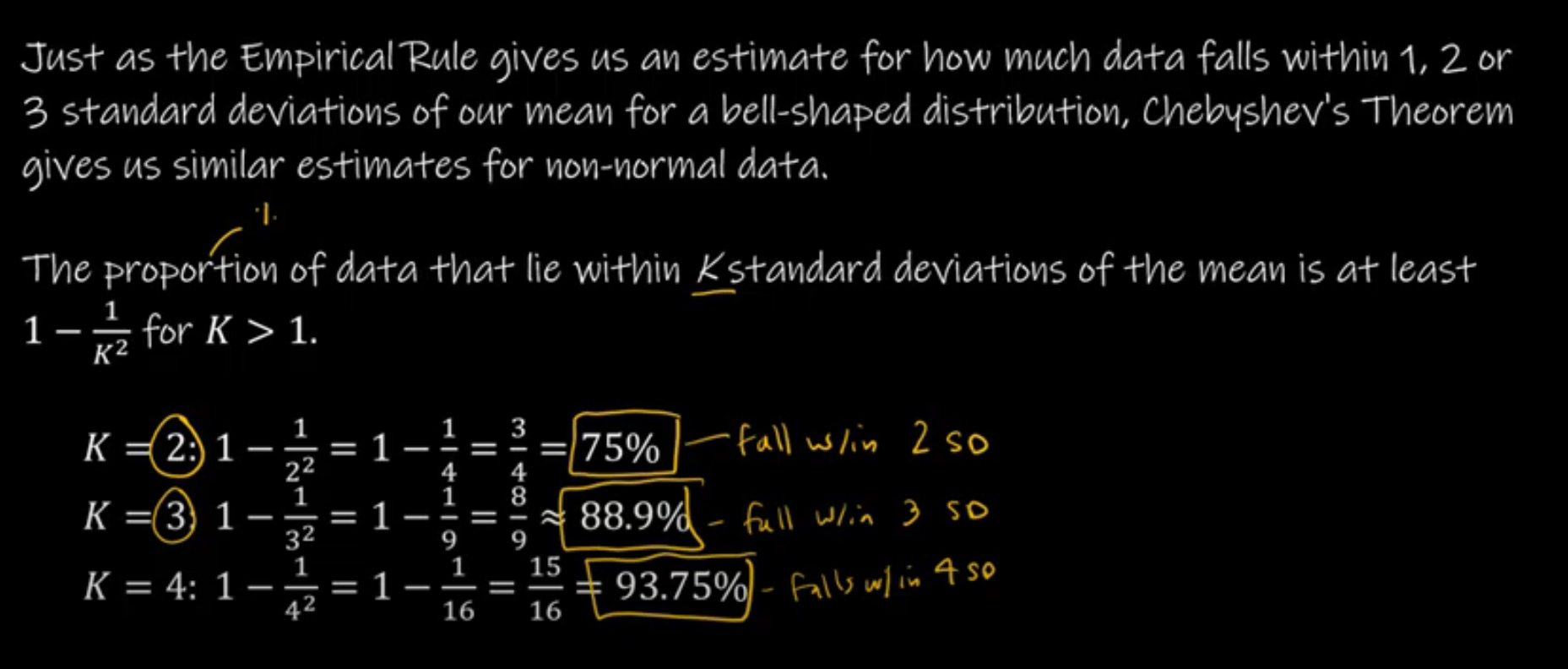
Chebyshev's InEquality:

if the dataset does not belong to a normal distribution with the help of Chebyshev's InEquality theorem we can find out how much percentage of data points will be falling within the range of standard deviation.

for better understanding watch this

Skewness:

Skewness, in statistics, is the degree of asymmetry observed in a probability distribution.

Distributions can exhibit right (positive) skewness or left (negative) skewness to varying degrees. A normal distribution (bell curve) exhibits zero skewness.

Kurtosis:

Kurtosis is a statistical measure used to describe the degree to which extreme values in either the tails or the peak of a frequency distribution.

There are three types of kurtosis: mesokurtic, leptokurtic, and platykurtic.

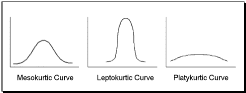
Mesokurtic: Distributions that are moderate in breadth and curves with a medium peaked height.

Leptokurtic: More values in the distribution tails and more values close to the mean (i.e. sharply peaked with heavy tails)

Platykurtic: Fewer values in the tails and fewer values close to the mean (i.e. the curve has a flat peak and has more dispersed scores with lighter tails).

This is the most foundational part of statistics, apart from the above key concepts two other key concepts are listed below considering the perceptive of data preprocessing and analysis.

Covariance

In simple terms, covariance is quantifying the relationship between two variables or columns in a particular data set.

Three types of covariance:

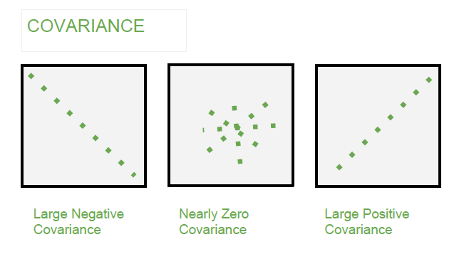
1. relationship with negative trends
2. relationship with no trends
3. relationship with positive trends

these positive and negative trends help us to identify the direction of the relationship. Even if covariance can be positive or negative still it can't tell you how much positive or how much negative or positive trend is.

For better understanding watch this

Correlation

Pearson Correlation Coefficient

(denoted by ρ)

the limitation of covariance is it can't tell you how much positive or how much negative or positive trend is to overcome we have Pearson Correlation Coefficient which helps us to find strength based on the variance of variables from your data, how strong those are correlated as well as the direction of the relationship.

when you are calculating the pearson correlation coefficient your value will lie between -1 and +1 always.

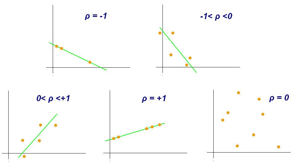
ρ = 1 : all data points fall in a straight line X(increase), Y(increase)

ρ = -1 : all data points fall in a straight line X(Decrease), Y(increase)

ρ = 0 : There is no relationship

-1 <= ρ => 0 : data points don't fall on straight line while X(Decrease), Y(increase)

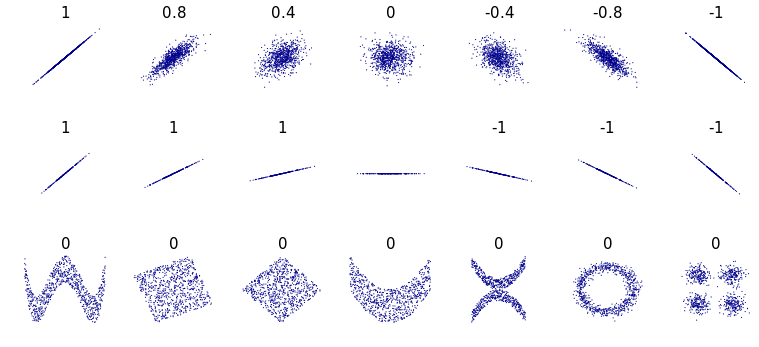
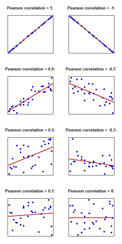
Covariance and Correlation are two terms that are exactly opposite to each other, they both are used in statistics and regression analysis, covariance shows us how the two variables vary from each other whereas correlation shows us the relationship between the two variables and how are they related.

Introduction to data types

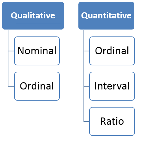
Nominal: Data at this level is categorized using names, labels, or qualities. eg: Brand Name, ZipCode, Gender.

Ordinal: Data at this level can be arranged in order or ranked and can be compared. eg: Grades, Star Reviews, Position in Race, Date

Interval: Data at this level can be ordered as it is in a range of values and meaningful differences between the data points can be calculated. eg: Temperature in Celsius, Year of Birth

Ratio: Data at this level is similar to interval level with the added property of an inherent zero. Mathematical calculations can be performed on these data points. eg: Height, Age, Weight

Hypothesis Testing

let us understand Hypothesis Testing by using a simple example.

Example: Class 8th has a mean score of 40 marks out of 100. The principal of the school decided that extra classes are necessary in order to improve the performance of the class. The class scored an average of 45 marks out of 100 after taking extra classes. Can we be sure whether the increase in marks is a result of extra classes or is it just random?

Hypothesis testing lets us identify that. It lets a sample statistic to be checked against a population statistic or statistic of another sample to study any intervention etc. Extra classes being the intervention in the above example.

Hypothesis testing is defined in two terms –

Null Hypothesis and Alternate Hypothesis.

Null Hypothesis being the sample statistic to be equal to the population statistic. For eg: The Null Hypothesis for the above example would be that the average marks after extra class are the same as those before the classes.

An Alternate Hypothesis for this example would be that the marks after extra class are significantly different from those before the class.

Hypothesis Testing is done on different levels of confidence and makes use of a z-score to calculate the probability. So for a 95% Confidence Interval, anything above the z-threshold for 95% would reject the null hypothesis.

Points to be noted:

We cannot accept the Null hypothesis, only reject it or fail to reject it. As a practical tip, the Null hypothesis is generally kept which we want to disprove. For eg: You want to prove that students performed better after taking extra classes on their exams. The Null Hypothesis, in this case, would be that the marks obtained after the classes are the same as before the classes.

Types of Errors in Hypothesis Testing

Now we have defined a basic Hypothesis Testing framework. It is important to look into some of the mistakes that are committed while performing Hypothesis Testing and try to classify those mistakes if possible.

Now, look at the Null Hypothesis definition above. What we notice at the first look is that it is a statement subjective to the tester like you and me and not a fact. That means there is a possibility that the Null Hypothesis can be true or false and we may end up committing some mistakes along the same lines.

There are two types of errors that are generally encountered while conducting Hypothesis Testing.

Type I error: Look at the following scenario – A male human tested positive for being pregnant. Is it even possible? This surely looks like a case of False Positive. More formally, it is defined as the incorrect rejection of a True Null Hypothesis. The Null Hypothesis, in this case, would be – Male Human is not pregnant.

Type II error: Look at another scenario where our Null Hypothesis is – A male human is pregnant and the test supports the Null Hypothesis. This looks like a case of False Negative. More formally it is defined as the acceptance of a false Null Hypothesis.

We have covered some basic yet fundamental statistical concepts. If you are working or plan to work in the field of data science, you are likely to encounter these concepts.

There is, of course, much more to learn about statistics. Once you understand the basics.

Thanks for reading✌, catch you in the next one.